-->

viernes, 17 de julio de 2020

Installing the Jupyter Software

 
Anaconda is a package manager, an environment manager, and Python distribution that contains a collection of many open source packages. An installation of Anaconda comes with many packages such as numpy, scikit-learn, scipy, and pandas preinstalled and is also the recommended way to install Jupyter Notebooks. This tutorial will include:


With that, let’s get started

Graphical Installation of Anaconda

Installing Anaconda using a graphical installer is probably the easiest way to install Anaconda.

1 ‒ Go to the Anaconda Website and choose a Python 3.x graphical installer (A) or a Python 2.x graphical installer (B). If you aren’t sure which Python version you want to install, choose Python 3. Do not choose both.


2 - Locate your download and double click it.


3 - Click on Continue

4 - Click on Continue
5 - Note that when you install Anaconda, it modifies your bash profile with either anaconda3 or anaconda2 depending on what Python version you choose. This can important for later. Click on Continue.
6 - Click on Continue to get the License Agreement to appear.
7 - Click on Install


8 - You’ll be prompted to give your password, which is usually the one that you also use to unlock your Mac when you start it up. After you enter your password, click on Install Software.

9 - Click on Continue. It is an Integrated Development Environment. You can learn about Python Integrated Development Environments here.


10 - You should get a screen saying the installation has completed. Close the installer and move it to the trash.


Test your Installation

1 - Open a new terminal on your Mac. You can do this by clicking on the Spotlight magnifying glass at the top right of the screen, type “terminal” then click on the terminal icon. Now, type the following command into your terminal

python --version


2 - Another good way to test your installation is to try and open a Jupyter Notebook. You can type the command below in your terminal to open a Jupyter Notebook. If the command fails, chances are that Anaconda isn’t in your path. See the next section on Common Issues.

jupyter notebook


The image below shows a Jupyter Notebook in action. terminal will open Safari asap. Jupyter notebooks contain both code and rich text elements, such as figures, links, and equations. You can learn more about Jupyter Notebooks here.


jueves, 12 de febrero de 2015

Gromacs Protein-Ligand Complex tutorial

When we are rocking in Gromacs there are a series of steps that we must follow:


Once you have downloaded the structure, you can visualize it using a viewing program such as VMD, Chimera, PyMOL.

we will prepare our system topology in two steps:
  1. Prepare the protein topology with pdb2gmx
  2. Prepare the ligand topology using external tools if applicable

The next command will create a topology file from selected PDB file in this case complex.pdb is our  PDB file, is a Protein bind to DNA. 


$ pdb2gmx -f complex.pdb

The structure will be processed by pdb2gmx, and you will be prompted to choose a force field:

Select the Force Field:
From '/usr/local/gromacs/share/gromacs/top':
 1: AMBER03 force field (Duan et al., J. Comp. Chem. 24, 1999-2012, 2003)
 2: AMBER94 force field (Cornell et al., JACS 117, 5179-5197, 1995)
 3: AMBER96 force field (Kollman et al., Acc. Chem. Res. 29, 461-469, 1996)
 4: AMBER99 force field (Wang et al., J. Comp. Chem. 21, 1049-1074, 2000)
 5: AMBER99SB force field (Hornak et al., Proteins 65, 712-725, 2006)
 6: AMBER99SB-ILDN force field (Lindorff-Larsen et al., Proteins 78, 1950-58, 2010)
 7: AMBERGS force field (Garcia & Sanbonmatsu, PNAS 99, 2782-2787, 2002)
 8: CHARMM27 all-atom force field (with CMAP) - version 2.0
 9: GROMOS96 43a1 force field
10: GROMOS96 43a2 force field (improved alkane dihedrals)
11: GROMOS96 45a3 force field (Schuler JCC 2001 22 1205)
12: GROMOS96 53a5 force field (JCC 2004 vol 25 pag 1656)
13: GROMOS96 53a6 force field (JCC 2004 vol 25 pag 1656)
14: OPLS-AA/L all-atom force field (2001 aminoacid dihedrals)
15: [DEPRECATED] Encad all-atom force field, using full solvent charges
16: [DEPRECATED] Encad all-atom force field, using scaled-down vacuum charges
17: [DEPRECATED] Gromacs force field (see manual)
18: [DEPRECATED] Gromacs force field with hydrogens for NMR

So we need to use a Force field (FF) which can handle protein and DNA molecules For this tutorial, we will use the  force field AMBER99SB-ILDN, so type 6 at the command prompt, followed by 'Enter'. The force field will contain the information that will be written to the topology. Chose wisely!

You will be prompted to choose a water model i chose TIP3.

There are many other options that can be passed to pdb2gmx. Some are listed here:
  • -ignh: Ignore H atoms in the PDB file; especially useful for NMR structures. Otherwise, if H atoms are present, they must be in the correct order and named exactly how GROMACS expects them to be.
  • -ter: Interactively assign charge states for N- and C-termini.
  • -inter: Interactively assign charge states for Glu, Asp, Lys, Arg, and His; assign disulfides to Cys.
You have now generated three new files: complex_processed.gro, topol.top, and posre.itp. complex_processed.gro is a GROMACS-formatted structure file that contains all the atoms defined within the force field (i.e., H atoms have been added to the amino acids in the protein). The topol.top file is the system topology. The posre.itp file contains information used to restrain the positions of heavy atoms.

The output shows electric charge and mass of the system by sections its really important to take note of the charge of each chain  protein or DNA. 

Processing chain 1 'A' (1262 atoms, 158 residues)
...
Total mass 17961.034 a.m.u.
Total charge 12.000 e

Processing chain 2 'B' (507 atoms, 25 residues)
...
Total mass 7605.906 a.m.u.
Total charge -24.000 e
Writing topology

Processing chain 3 'C' (491 atoms, 24 residues)
...
Total mass 7351.772 a.m.u.
Total charge -23.000 e

Total mass in system 32918.712 a.m.u.
Total charge in system -35.000 e

It is possible to simulate proteins and other molecules in different solvents, provided that good parameters are available for all species involved.
There are two steps to defining the box and filling it with solvent:
  1. Define the box dimensions using editconf.
  2. Fill the box with water using genbox.
As you become more comfortable with periodic boundary conditions and box types, I highly recommend the rhombic dodecahedron, as its volume is ~71% of the cubic box of the same periodic distance, thus saving on the number of water molecules that need to be added to solvate the protein. For an excellent summary of the many different water models, click here, but be aware that not all of these models are present within GROMACS.

Let's define the box using editconf:


$ editconf -f conf.gro -o complex_newbox.gro -c -bt dodecahedron -d 1.0

Now that we have defined a box, we can fill it with solvent (water). Solvation is accomplished using genbox:

$ genbox -cp complex_newbox.gro -cs spc216.gro -o complex_solv.gro -p topol.top  


What genbox has done is keep track of how many water molecules it has added, which it then writes to your topology to reflect the changes that have been made. Note that if you use any other (non-water) solvent, genbox will not make these changes to your topology! Its compatibility with updating water molecules is hard-coded


We now have a solvated system that contains a charged protein. The output of pdb2gmx told us that the protein has a net charge of -35e (based on its amino acid composition). If you missed this information in the pdb2gmx output, look at the last line of your [ atoms ] directive in topol.top; it should read (in part) "qtot 6." Since life does not exist at a net charge, we must add ions to our system.
The tool for adding ions within GROMACS is called genion. What genion does is read through the topology and replace water molecules with the ions that the user specifies. The input is called a run input file, which has an extension of .tpr; this file is produced by the GROMACS tool grompp (GROMACS pre-processor), which will also be used later when we run our first simulation. What grompp does is process the coordinate file and topology (which describes the molecules) to generate an atomic-level input (.tpr). The .tpr file contains all the parameters for all of the atoms in the system.
Use grompp to assemble a .tpr file, using any .mdp file. I use an .mdp file for running energy minimization, since they require the fewest parameters and are thus the easiest to maintain. To produce a .tpr file with grompp, we will need an additional input file, with the extension .mdp (molecular dynamics parameter file); grompp will assemble the parameters specified in the .mdp file with the coordinates and topology information to generate a .tpr file.

An .mdp file is normally used to run energy minimization or an MD simulation, but in this case is simply used to generate an atomic description of the system. An example .mdp file (the one we will use) can be downloaded here.
In reality, the .mdp file used at this step can contain any legitimate combination of parameters. I typically use an energy-minimization script, because they are very basic and do not involve any complicated parameter combinations.
Assemble your .tpr file with the following:
$ grompp -f ions.mdp -c complex_solv.gro -p topol.top -o ions.tpr

Now we have an atomic-level description of our system in the binary file ions.tpr. We will pass this file to genion:
$ genion -s ions.tpr -o complex_solv_ions.gro -p topol.top -pname NA -nname CL -np 35


When prompted, choose group 14 "SOL" (for this case) for embedding ions. You do not want to replace parts of your protein with ions.
In the genion command, we provide the structure/state file (-s) as input, generate a .gro file as output (-o), process the topology (-p) to reflect the removal of water molecules and addition of ions, define positive and negative ion names (-pname and -nname, respectively), and tell genion to add only the ions necessary to neutralize the net charge on the protein by adding the correct number of negative ions (-nn 8). You could also use genion to add a specified concentration of ions in addition to simply neutralizing the system by specifying the -neutral and -conc options in conjunction. Refer to the genion man page for information on how to use these options.
The names of the ions specified with -pname and -nname were force field-specific in previous versions of GROMACS, but have been standardized as of version 4.5. The specified ion names are always the elemental symbol in all capital letters, which is the [ moleculetype ] name that is then written to the topology. Residue or atom names may or may not append the sign of the charge (+/-), depending on the force field. Do not use atom or residue names in the genion command, or you will encounter errors in subsequent steps.

The solvated, electroneutral system is now assembled. Before we can begin dynamics, we must ensure that the system has no steric clashes or inappropriate geometry. The structure is relaxed through a process called energy minimization (EM).
The process for EM is much like the addition of ions. We are once again going to use grompp to assemble the structure, topology, and simulation parameters into a binary input file (.tpr), but this time, instead of passing the .tpr to genion, we will run the energy minimization through the GROMACS MD engine, mdrun.
Assemble the binary input using grompp using this input parameter file:
grompp -f minim.mdp -c complex_solv_ions.gro -p topol.top -o em.tpr

Make sure you have been updating your topol.top file when running genbox and genion, or else you will get lots of nasty error messages ("number of coordinates in coordinate file does not match topology," etc).
We are now ready to invoke mdrun to carry out the EM:
mdrun -v -deffnm em

The -v flag is for the impatient: it makes mdrun verbose, such that it prints its progress to the screen at every step. The -deffnm flag will define the file names of the input and output. So, if you did not name your grompp output "em.tpr," you will have to explicitly specify its name with the mdrun -s flag. In our case, we will get the following files:
  • em.log: ASCII-text log file of the EM process
  • em.edr: Binary energy file
  • em.trr: Binary full-precision trajectory
  • em.gro: Energy-minimized structure
writing lowest energy coordinates.

Steepest Descents converged to Fmax < 1000 in 1671 steps
Potential Energy  = -1.4910198e+06
Maximum force     =  8.8282404e+02 on atom 123
Norm of force     =  1.2215010e+01
There are two very important factors to evaluate to determine if EM was successful. The first is the potential energy (printed at the end of the EM process, even without -v). Epot should be negative, and (for a simple protein in water) on the order of 105-106, depending on the system size and number of water molecules. The second important feature is the maximum force, Fmax, the target for which was set in minim.mdp - "emtol = 1000.0" - indicating a target Fmax of no greater than 1000 kJ mol-1 nm-1. It is possible to arrive at a reasonable Epot with Fmax > emtol. If this happens, your system may not be stable enough for simulation. Evaluate why it may be happening, and perhaps change your minimization parameters (integrator, emstep, etc).
Let's do a bit of analysis. The em.edr file contains all of the energy terms that GROMACS collects during EM. You can analyze any .edr file using the GROMACS tools g_energy:
g_energy -f em.edr -o potential.xvg
At the prompt, type "10 0" to select Potential (10); zero (0) terminates input. You will be shown the average of Epot, and a file called "potential.xvg" will be written. To plot this data, you will need the Xmgrace plotting tool. The resulting plot should look something like this, demonstrating the nice, steady convergence of Epot:
Statistics over 1670 steps [ 1.0000 through 1670.0000 ps ], 1 data sets
All statistics are over 1322 points (frames)

Energy                      Average   Err.Est.       RMSD  Tot-Drift
-------------------------------------------------------------------------------
Potential                -1.44656e+06      24000    71431.2    -155083  (kJ/mol)
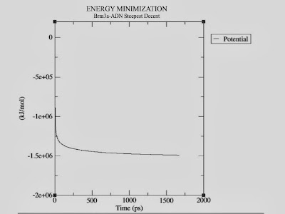
Energy Minimization plot
Now that our system is at an energy minimum, we can begin real dynamics.

EM ensured that we have a reasonable starting structure, in terms of geometry and solvent orientation. To begin real dynamics, we must equilibrate the solvent and ions around the protein. If we were to attempt unrestrained dynamics at this point, the system may collapse. The reason is that the solvent is mostly optimized within itself, and not necessarily with the solute. It needs to be brought to the temperature we wish to simulate and establish the proper orientation about the solute (the protein). After we arrive at the correct temperature (based on kinetic energies), we will apply pressure to the system until it reaches the proper density.
Remember that posre.itp file that pdb2gmx generated a long time ago? We're going to use it now. The purpose of posre.itp is to apply a position restraining force on the heavy atoms of the protein (anything that is not a hydrogen). Movement is permitted, but only after overcoming a substantial energy penalty. The utility of position restraints is that they allow us to equilibrate our solvent around our protein, without the added variable of structural changes in the protein.
Equilibration is often conducted in two phases. The first phase is conducted under an NVT ensemble (constant Number of particles, Volume, and Temperature). This ensemble is also referred to as "isothermal-isochoric" or "canonical." The timeframe for such a procedure is dependent upon the contents of the system, but in NVT, the temperature of the system should reach a plateau at the desired value. If the temperature has not yet stabilized, additional time will be required. Typically, 50-100 ps should suffice, and we will conduct a 100-ps NVT equilibration for this exercise. Depending on your machine, this may take a while (just over an hour on a dual-core MacBook). Get the .mdp file here.
We will call grompp and mdrun just as we did at the EM step:
grompp -f nvt.mdp -c em.gro -p topol.top -o nvt.tpr

mdrun -deffnm nvt

A full explanation of the parameters used can be found in the GROMACS manual, in addition to the comments provided. Take note of a few parameters in the .mdp file:
  • gen_vel = yes: Initiates velocity generation. Using different random seeds (gen_seed) gives different initial velocities, and thus multiple (different) simulations can be conducted from the same starting structure.
  • tcoupl = V-rescale: The velocity rescaling thermostat is an improvement upon the Berendsen weak coupling method, which did not reproduce a correct kinetic ensemble.
  • pcoupl = no: Pressure coupling is not applied.
Let's analyze the temperature progression, again using g_energy:
g_energy -f nvt.edr


miércoles, 18 de enero de 2012

Python programming in Mac

Python is a general-purpose, high-level programming language whose design philosophy emphasizes code readability. Python claims to combine "remarkable power with very clear syntax", and its standard library is large and comprehensive. Its use of indentation for block delimiters is unique among popular programming languages.
For these reasons is one of the best tools for programing in bioinformatics for beggines because there´s a lot of modules for bioinformatic tools as NumPySciPyBioPython and more. also you can get it typing in your comand line if you already have installed Xcode for mac strongly recomended , if you dont have it download Fink
Python is actually included in Mac OS X, open your terminal and tipe  python to call enviroment:


Comand  $ python   will open the enviroment and show installed version in your OS X. for know where is the directory just tipe: 


$ which python
But if your are plannig to move to the latest version you can install it if your have administrator's rights to do this. On a Unix style system this is normally done by:

$ sudo easy_install  biopython
Whit fink you can tipe in terminal line:


$ sudo apt-get install python-biopython
This is the fist program i create in python is for calculate Velocity in enzymatic reaction from  Michaelis–Menten kinetics is one of the simplest and best-known models of enzyme kinetics. It is named after German biochemist Leonor Michaelis and Canadian physician Maud Menten. The model takes the form of an equation describing the rate of enzymatic reactions, by relating reaction rate v to [S], the concentration of a substrate S. Its formula is given by:


CODE:

#! /Usr/bin/python

from math import*

# v= Vmax(S)/Km+(S)

Vmax= float(raw_input('Vmax: '))
S= float(raw_input('S: '))
Km= float(raw_input('Km: '))
Velocity=(Vmax*(S))/(Km+S)

print Velocity

# Author: Alejandro Rendon 

jueves, 12 de enero de 2012

Write modeller scripts in MAC


MODELLER is a software used for homology or comparative modeling of protein three-dimensional structures,  The user provides an alignment of a sequence to be modeled with known related structures and MODELLER automatically calculates a model containing all non-hydrogen atoms. so we have to add Hydrogen atoms after calculate our modell. Following tutorial is easy to create and install modeller, sometimes is necesary to download Python package and we need a compiler to install packages easily for this reason we need to intall X code our use another compiler. 
To download modeller just click in the link: Modeller

Note: cd command will allow you to change directories. When you open a terminal you will be in your home directory. 

To run modeller open terminal:

Once installed the package of modeller access through terminal whit the comand cd if your folder of scripts is in desk example tipe:
  
$ cd Desktop

then you will be in the folder Desktop after this access to your folder 

$ cd Proteinx

as an example this is my terminal line

macbook-de-fixxer-2:~ javier$ cd Desktop
macbook-de-fixxer-2:Desktop javier$ cd cryo-em

once you are in the rigth folder to run modeller comands use the comand mod9.9 to call the enviroment of modeller:

macbook-de-fixxer-2:cryo-em javier$ mod9.9

and after the comand to call modeller pack write the script you wan to run example:


macbook-de-fixxer-2:cryo-em javier$ mod9.9 build_profile.py

miércoles, 11 de enero de 2012

Installing Xcode and Compiling Objective-C on Mac OS X


If you are planning to develop Mac OS x applications (even iPhone or iPad applications for that matter), however, you are going to need to use an Intel based Mac OS X system at some point in the future.
Perhaps the biggest advantage of using Mac OS X as your Objective-C learning platform (aside from the ability to develop iPhone and Mac OS X applications) is the fact that you get to use Apple's Xcode development tool. Xcode is a powerful and easy to use development environment that is available free of charge to anyone fortunate enough to own an Apple computer running Mac OS X.
Just click in the link to get the info:

Mac OS X install pytables and h5py

  1. Install tables - need NumPy version 1.6
  2. Get NumPy from sourceforge and install - need Python 2.7
  3. Install python 2.7 on Lion, open new terminal (or refresh path)
  4. curl http://python-distribute.org/distribute_setup.py | python
  5. curl https://raw.github.com/pypa/pip/master/contrib/get-pip.py | python
  6. sudo pip install ipython
  7. sudo pip install tables
  8. need numexpr > 1.4.1, 
  9. Download anc ompile numexpr -> wants to compile using gcc-4.2
  10. sudo ln -s gcc gcc-4.2
  11. sudo pip install cython
  12. Get HDf5 from http://www.hdfgroup.org/ftp/HDF5/current/bin/mac-intel-x86_64/hdf5-1.8.8-mac-intel-x86_64-shared.tar.gz
  13. /configure and compile
  14. Copy the hdf5 folder whereever you want
  15. python setup.py build --hdf5=/path/to/hdf5 (from the unzipped source of h5py)
  16. sudo python setup.py install --hdf5=/usr/local/hdf5/ (in the unzipped dir of pytables)
In contrast, to get h5py working on Ubuntu:


sudo apt-get install libhdf5-serial-dev
 
sudo easy_install h5py